Simple Spatial Experiments

The project described here is a simple data recording program for the Phidget Spatial. We play with the program and record data to learn things about our environment.

Practical concepts covered are (click on links to see other projects on that topic): Data Logging Writing to a text file Using Phidgets with C/C++ Analyzing your Phidget Data

As with any of our described projects, Phidgets takes care of the electrical component design. Here, we also provide some simple code so you can play around with your Spatial and save the data to plot later.

Time:	About two hours
Special Needed Tools:	None
Materials and Phidgets:	A Phidget Spatial, USB cord, and your computer

You should also have:

• Already worked through our Phidget Spatial Getting Started Guide for your Spatial Device, found in its user guide - this will show you how to get the the Phidget Libraries installed for your operating system.
• A a C compiler we support (including gcc, MinGW, Borland, Visual Studio, and many more) on your computer
• If you would like to follow along with the graphing examples, you can install the R Statistical package, which is free and available for Windows, Mac, and Linux.

Introduction

A Phidget Spatial can measure acceleration, and some models can also measure gyroscopic motion and magnetic fields.

We start with a Phidget spatial just on our desk, and then play around with it and plot the data.

Phidgets

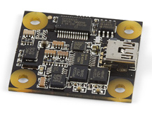
All you need is a Phidget Spatial - this page shows use of the 1056 - PhidgetSpatial 3/3/3. Hook it up using USB to your computer as shown in the getting started guide for your Spatial. (This can be found in its user guide.)

Code

Our code measures data by writing it every time we have a 'new data' event. Here we call the function that handles that event SpatialDataHandler. That function receives an event at the default timing (about every 8 ms) and then writes the received data to a file called spatial_data.csv.

You can either peruse the code and modify it to your needs, or simply copy and paste it into a file. We called our file sample_code.c.

#include <stdio.h>
#include <stdlib.h>
#include "phidget21.h"

#ifndef _WIN32 
#define __stdcall
#endif

// Our function that gets called at the set data rate (default of 8 ms)
// Different rates can be set using CPhidgetSpatialHandle_setDataRate(milliseconds)
int __stdcall SpatialDataHandler(CPhidgetSpatialHandle spatial, void *userptr, CPhidgetSpatial_SpatialEventDataHandle *data, int count)
{
    int i;
    printf(".");
    fflush(stdout);
    // Sometimes we get more than one packet per event, this counts through them
    for(i = 0; i < count; i++) {
        FILE *file = (FILE *) userptr;
        // Our header was already printed on opening the file: 
        // Timestamp, then Accel X,Y,Z, then Ang Rate X,Y,Z then Mag Field X,Y,Z
        fprintf(file, "%f,", data[i]->timestamp.seconds + (data[i]->timestamp.microseconds)/1000000.0);
        fprintf(file, "%6f,%6f,%6f,", data[i]->acceleration[0], data[i]->acceleration[1], data[i]->acceleration[2]);
        fprintf(file, "%6f,%6f,%6f,", data[i]->angularRate[0], data[i]->angularRate[1], data[i]->angularRate[2]);
        // Due to time for internal calibration, the compass sometimes returns the large constant PUNK_DBL
        if (data[i]->magneticField[0] == PUNK_DBL) {
	    fprintf(file, "%6f,%6f,%6f\n", 0.0, 0.0, 0.0);
        } else {
    	    fprintf(file, "%6f,%6f,%6f\n", data[i]->magneticField[0], data[i]->magneticField[1], data[i]->magneticField[2]);
        }
        fflush(file);
    }
    return 0;
}

int main(int argc, char* argv[]) {

    int result;
    char character;

    FILE *file = fopen("spatial_data.csv","w");

	CPhidgetSpatialHandle spatial = 0;

    // Print the header at the top of the file
    fprintf(file, "Time,Accel_X,Accel_Y,Accel_Z,Ang_X,Ang_Y,Ang_Z,Mag_X,Mag_Y,Mag_Z\n");

    CPhidgetSpatial_create(&spatial);

    // Hook our file-writing function above into the data stream events
    CPhidgetSpatial_set_OnSpatialData_Handler(spatial, SpatialDataHandler, (void *) file);

    CPhidget_open((CPhidgetHandle)spatial, -1);

    result = CPhidget_waitForAttachment((CPhidgetHandle)spatial, 10000);
    if (result) {
        printf("No Device!\n");
        return 0;
    }

    printf("Press Enter to end\n");
    getchar();

    CPhidget_close((CPhidgetHandle)spatial);
    CPhidget_delete((CPhidgetHandle)spatial);
    fclose(file);
    return 0;
}

Compile your C file using the instructions for our examples on the Language - C/C++ page.

• This code was written for gcc, so you'll either have to use a gcc compiler (Cygwin, Mac OSX, or Linux) or modify the code to work with your favourite platform.
• The code has been tested on Linux, and Cygwin on Windows.
• Make sure to copy the last blank line return at the end of the file - many Windows compilers insist on this being present.

Then, run your program in a command line manner, so you can input a keystroke and Enter to end the program. If you:

1. Have your spatial plugged in
2. Lie the spatial down flat (chips up) on the same surface as your computer keyboard
3. Compile the sample_code.c file using the source code above
4. Use gcc on Mac OS, Linux, or Cygwin, and then
5. Run the program for about three seconds before pressing a key (and Enter) to exit

...It might look something like this:

Putting it All Together

Running the program as described in the Code section above will give you a file called spatial_data.csv in the same folder as your source code.

The file is a Comma-Separated-Value (csv) file, and can be easily imported into a spreadsheet by using a comma character as a separator. Often, your default installed spreadsheet program (such as Microsoft Office Excel) will automatically detect that the csv file should be opened into a spreadsheet:

You can then make your own plots on the spreadsheet. Or, you can install the R Statistical package, which is free and available for Windows, Mac, and Linux, and follow along making these graphs as well....

If you start R in the same directory as your code and data (for example, on the DOS prompt going to that directory and typing "R"), you can then import the data file like this:

data = read.csv("spatial_data.csv")

You can then access each column of data using a "$" separator. For example, data$Accel_X is the column of X-axis acceleration data.

Since it is the Z axis that is feeling the effects of gravity's pull (which is itself acceleration), we can plot the Z-axis acceleration versus Time in R like this:

plot(data$Time,data$Accel_Z)

Or we can pretty it up with connecting lines, some colour, and some axis labels like this:

plot(data$Time,data$Accel_Z,type="l",xlab="Time in Seconds",ylab="Z Axis Acceleration",col="blue")

...Which produces a graph like this of our three seconds of recording:

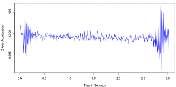
Even from this little three second experiment, we have a number of events and data boundaries:

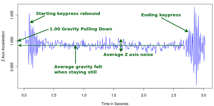
If both your keyboard and your spatial are on a shared and sufficiently hard surface, the force from your key presses starting and ending the program in a command line prompt will vibrate down the table and show up as acceleration. Force equals mass times acceleration, so applying a force to the keys, and there to the table, and there to the Spatial will create acceleration in the Spatial.

You will also notice that there is some small up and down between key presses. This gives us both:

• The average noise (as long as your table is completely still and untouched), and
• The average sensed gravity along the Z axis

You may also note that the sensed acceleration is very slightly off of one gravity in the Z direction. Gravity varies very slightly naturally over the Earth. However, before you go brushing off a deviation from 1.00 as due to natural variation, we want to make sure we have no tilt. Examining the Spatial on your desk may reveal something like this:

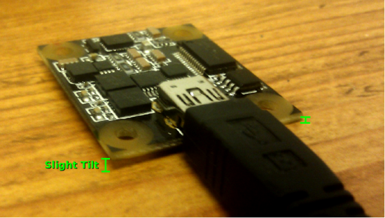
Using the user guide for the spatial, we can use the equation for tilt to calculate tilt for each time point in R (the 180 over 3.14 is to convert from radians to degrees):

tilt = 180/3.14 * (asin(data$Accel_X) + asin(data$Accel_Y))

And plotting this data (with some colour and labels) by using:

plot(data$Time,tilt,type="l",xlab="Time in Seconds",ylab="Tilt",col="orange")

....Gives:

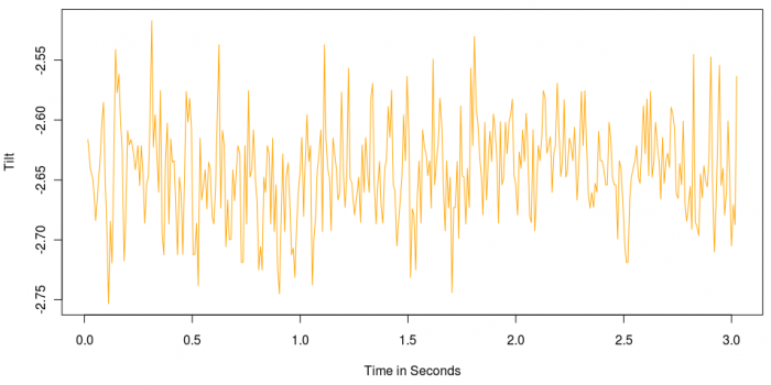
We can see that the tilt doesn't really vary much at 0 and 3 seconds when our key presses occurred. So the up and down is probably mostly due to axis noise. This means we're mostly interested in the average tilt on the table rather than the constant fluctuation.

Finding an average tilt value over these three seconds by:

sum(tilt)/length(tilt)

Gives an average tilt in our data of -2.6 degrees, which is reasonable for what we saw in the photo of the Spatial on our desk.

Extra Credit

Use the datalogger program to:

• Record vibrations when the Spatial is on a humming device (your computer, your fridge, etc) - compare with a still desk
• Measure rotation using the Gyroscope if one is on your Spatial
• Record acceleration while you move the Spatial (without rotating) a known distance
  • Try to reverse-derive this distance (position change) from the acceleration data alone (it is hard!)
  • Move the accelerometer quickly and slowly along this distance and see how it becomes easier or harder to measure
  • Think about leaving the accelerometer still for a little while to measure noise, and then moving it

And so on. Capturing data and plotting it can be a powerful first step before using that data to actually perform additional tasks.